Most Snowflake accounts don’t get optimized until someone complains. Finance flags the bill, or a data analyst says a dashboard is too slow. Only then does anyone open the query profile.
That was one of the first points raised in a recent webinar hosted by Yuki’s CEO Amir and Samer, Solutions Engineer at Snowflake. The session ran 15 minutes past the scheduled end because the two of them kept going deeper into the architectural mechanics that actually affect Snowflake performance and cost, past the generic advice most teams have already heard.
Below is a recap organized the way the session was structured: architectural foundations first, then ingestion, then transformations, then consumption.
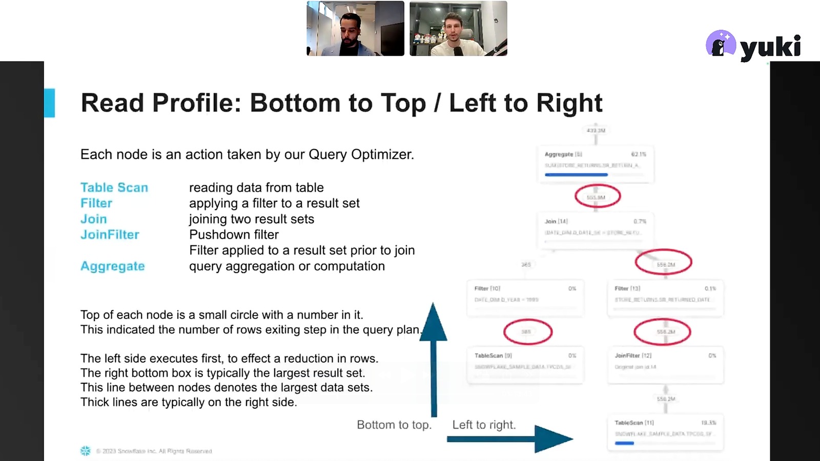
Read the Query Profile Bottom to Top
Before optimizing anything, you need a way to measure it. That’s the query profile, found under Monitor > History in Snowsight.
Most people read it top to bottom. That’s backwards. Start at the bottom, since that’s where the table scan happens, the first real step in processing the data. Read left to right too: small data volumes on the left, larger ones on the right as the query progresses.
One metric to watch for: bytes spilled to local storage. It means compute and memory weren’t enough, so Snowflake is writing to SSD. If you see bytes spilled to remote storage, it’s worse: local disk wasn’t enough either, so data is spilling to cloud storage. Either one is a clear sign of a performance and cost problem, not something to leave alone.
The instinct at this point is usually to add a clustering key. Don’t start there. As Samer put it, clustering and similar tuning features are “putting a plaster on the wound.” Re-examine the table architecture first. Clustering is a second step, after you’ve confirmed the underlying design is actually sound.
Micro-Partitions: The Concept Everything Else Depends On
This is the part of the webinar worth watching in full. Clustering, dynamic tables, and Gen2 warehouses only make sense once you understand micro-partitions.
Here’s the mechanic. Load 10 million rows into Snowflake and they don’t land as one object. Snowflake automatically splits them into small immutable files, each holding a slice of the rows, called micro-partitions. At the same time, it stores metadata about each partition (min values, max values, distinct values) in what’s called the cloud services layer. The actual data sits in the storage layer. Queries run in the compute layer.
When a query with a WHERE clause comes in, the cloud services layer checks the metadata first and figures out which micro-partitions could possibly contain matching rows. Only those get pulled into compute. That’s how a query profile ends up showing something like “2 partitions scanned out of 10,000 total”: the filtering already happened in metadata, before any compute was spent.
This is also why compilation time isn’t billed like warehouse compute. The work of narrowing down partitions happens before the warehouse does any real processing, and it’s billed separately (and much more cheaply) than compute time. If a query profile shows five minutes of a ten-minute runtime going to compilation, that’s worth digging into on its own.
One more property matters more than most people expect: micro-partitions are immutable. An update or delete doesn’t touch a row in place. It deletes the whole micro-partition and writes a new one. A full table reload rewrites everything. An incremental load is cheaper, since only the changed micro-partitions get rewritten. The trap is a “scattered” incremental load: a small number of changes landing across a large number of different micro-partitions, common with SCD Type 2 dimensions, which forces a rewrite that behaves almost like a full reload even though the actual row count changed is small.
Natural clustering (data ordered the way it arrives, usually by time) is enough for most tables. A clustering key is only needed when query patterns don’t line up with that natural order, for example filtering by sensor location instead of by timestamp.
Optimizing Ingestion: Stop Doing Row-by-Row Inserts
Ingestion optimization has the smallest impact on the bill of the three areas covered, but it’s the easiest fix.
The biggest anti-pattern flagged in the session: row-by-row INSERT INTO statements. Whether that’s a Python script pushing rows one at a time, or a legacy ETL tool doing the same thing under the hood, it spins up a warehouse for work that doesn’t need one. The fix is Snowpipe Streaming: no warehouse required, roughly 0.0037 credits per gigabyte, over 10 GB per second throughput, and 5 to 10 second latency. Available via REST API, Java SDK, or Python SDK.
No streaming use case? A scheduled COPY INTO beats row-by-row inserts, but Snowpipe is the better default for batch loads landing in external cloud storage. It triggers automatically on file arrival, doesn’t need a running warehouse, and costs the same 0.0037 credits per gigabyte.
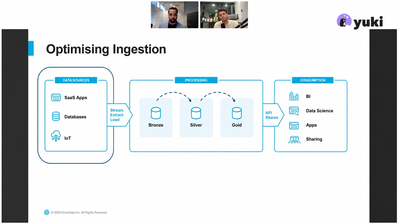
The last ingestion anti-pattern: skipping the Medallion architecture, meaning data lands in bronze and gets queried directly instead of moving through silver and gold. This came up as one of the most common causes of excessive micro-partition scanning. A related mistake is transforming data outside Snowflake before loading it, an ETL pattern instead of ELT. Transformation is cheap inside Snowflake, and pre-transforming externally tends to break natural clustering on the way in, which defeats the point.
Worth checking before chasing “real-time” anything: does the business actually need it? A lot of “we need real-time” requests fall apart once you ask what changes if refresh happens every five minutes instead of every second. Unnecessary real-time pipelines cost more in compute, complexity, and architecture than the use case justifies.
Optimizing Transformations: Two Goals
Transformation is where the real cost and performance gains live, once ingestion is out of the way. The framing from the session: there are two goals, minimize the number of micro-partitions read, and minimize the number written.
For reads: CREATE TABLE AS SELECT, INSERT OVERWRITE, or a dbt table materialization all mean a full refresh, reading and rewriting every micro-partition every time. The fix in most cases is dynamic tables. Take the same SELECT statement already in use and put it in a dynamic table; Snowflake builds the incremental pipeline underneath it automatically.
For writes: if the pipeline is already incremental but write volume is still high, look for scattered incremental loads, usually hiding in merge statements, updates, and deletes spread across a large number of micro-partitions. This is where Gen2 warehouses help. Standard warehouses use a copy-on-write model. Gen2 warehouses ship with software optimizations that push Snowflake closer to a merge-on-read pattern for DML-heavy workloads. One example from the session, a case that circulated on LinkedIn: switching a DML-heavy job to Gen2 cut runtime from 43 minutes to 14 minutes and reduced data written from 334 GB to 42 GB.
Gen2 warehouses run roughly 25 to 30 percent more than Gen1, which sets a clear bar. If moving a DML-heavy workload to Gen2 doesn’t save at least that much in runtime, it’s not a cost win, though it may still be worth it if speed is the actual priority. The test costs nothing: spin up a Gen2 warehouse, run the same query, compare.
Warehouse Sizing Is a Concurrency Problem
This part covered something most Snowflake content skips: degree of parallelism (DOP), the score Snowflake assigns each query based on how many resources it needs. A complex query might get a DOP of 8. A small one, a DOP of 1.
Default warehouse concurrency is 8, meaning up to eight queries with a DOP of 1 can run at once before others start queuing. That gives you two signals to act on:
- Small number of concurrent queries, everything else stuck in a queue: fix is warehouse size (scale up).
- A lot of small queries queuing at once: fix is cluster count (scale out), and with Snowflake’s larger multi-cluster support this is more accessible than it used to be.
The mistake called out repeatedly in the session: teams scale cluster size hoping it’ll speed up a job when the bottleneck was warehouse size, or the reverse. One real dbt example: three models running for 10, 7, and 8 minutes turned out to be competing for resources on the same warehouse at the same time. Splitting them across separate warehouses got the team to their 5-minute SLA. In another case, bumping warehouse size up one tier cut total runtime by roughly 40 percent at a higher cost, a fair tradeoff when the SLA calls for it.
There’s also a warehouse-level concurrency parameter, separate from cluster count, that goes from a default of 8 up to 32. Useful for high-volume, low-complexity ingestion workloads, but it needs ongoing monitoring, not a set-and-forget change.
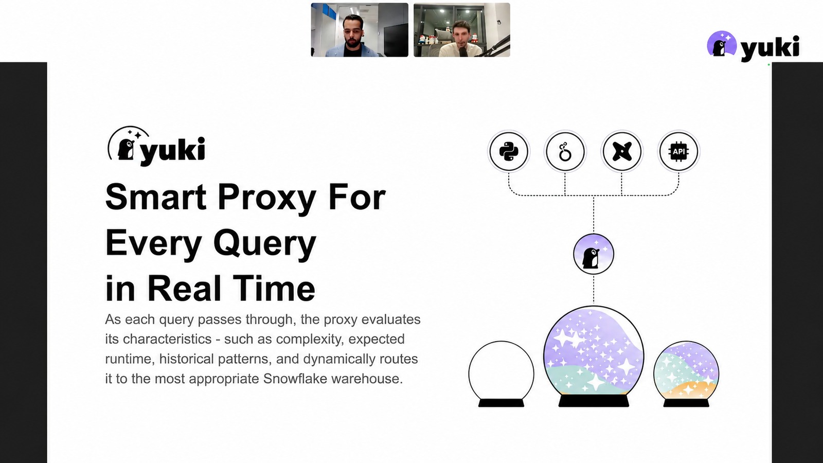
This kind of query-by-query, warehouse-by-warehouse tuning is exactly the manual work that stops scaling once a data team grows past a certain size. It’s the problem Yuki was built around: a proxy sitting between your tools (dbt, APIs, scripts) and Snowflake that picks the right warehouse size, type, and availability for every query in real time. Teams using it have gone from around 15 percent warehouse utilization to close to 95, without anyone manually reassigning workloads.
Optimizing Consumption: Views, Real-Time Tables, Transactional Workloads
The last part of the session covered where end users actually feel Snowflake’s performance: consumption.
BI tool queries are a common pain point. Legacy BI tools especially tend to generate complex, repetitive queries that recompute the same aggregation over and over. Materialized views fix this without touching anything on the BI side. Create a materialized view filtered on whatever a team queries repeatedly (the webinar used a “cat sales” example), and Snowflake automatically reroutes matching queries against the base table to the materialized view. End users don’t need to know it exists or point their BI tool at it directly.
For real-time, high-volume, low-latency workloads (crypto trading dashboards, customer-facing analytics that can’t wait 10 to 20 seconds), standard warehouses aren’t the right engine. Interactive tables add extra metadata on top of the micro-partition model to speed up queries, paired with an always-on interactive warehouse with a pre-warmed cache, at up to 40 percent lower cost than a comparable regular warehouse for that workload. Query latency on interactive tables is capped at five seconds, so it’s worth confirming the workload actually fits before adopting it. Streaming ingestion directly into interactive tables is currently in private preview.
For transactional workloads (a SaaS product serving row-level reads and writes, a voice agent that needs sub-second responses), analytical engines aren’t a fit no matter how well tuned. That’s what Snowflake Postgres is for: a genuinely different engine built for row-by-row access instead of columnar analytics.
The rough mental model: standard warehouses for analytics, interactive tables for high-volume real-time analytics, Snowflake Postgres for transactional workloads, and hybrid workloads increasingly sitting somewhere in between.
The Compute Crisis Nobody’s Ready For
The closing part of the webinar is the one worth remembering. Up through roughly 2022, most companies were focused on adoption: getting onto Snowflake, building out pipelines. From 2023 to 2025, focus shifted to optimization: tuning warehouses, adopting Iceberg, cleaning up what had already been built.
Now every team is connecting AI agents and AI workloads to their data cloud, and query volume from those workloads doesn’t behave like traditional BI traffic. It’s less predictable and growing fast, and most data teams don’t have the compute management practices in place yet to handle it. Snowflake is a good fit for analytical AI workloads, but the compute discipline needed to run them efficiently at scale is a different problem than most teams have already solved.
That’s the gap Yuki is built to close: automated, per-query compute optimization that keeps Snowflake efficient as workloads (including AI-driven ones) keep growing, without turning every warehouse-sizing decision into a manual investigation.
Want the Technical Deep Dive?
This recap covers the key takeaways, but the full webinar goes deeper into the live-drawn architecture walkthrough, real customer utilization numbers, and audience Q&A.
If your team is dealing with spilled queries, ballooning DML costs, or a warehouse fleet nobody’s sure is sized correctly, start a free trial or request a free cost analysis to see where your Snowflake spend is actually going.